Pure lambda calculus has encodings for many different data structures like lists, numbers, strings, and trees. Wrapped in monadic IO, lambda calculus provides a great interface for computation – as can be seen in user-friendly syntactic variants like my programming language bruijn. Such simple languages, however, typically don’t support graphical output (aside from ASCII art).

I present the “Lambda Screen”, a way to use terms of pure lambda calculus for generating images. I also show how recursive terms (induced by fixed-point combinators) can lead to infinitely detailed fractals.

If you want to skip the details or want to figure out its inner workings yourself, go to my reference implementation (source-code) and flip through the examples.

Encoding

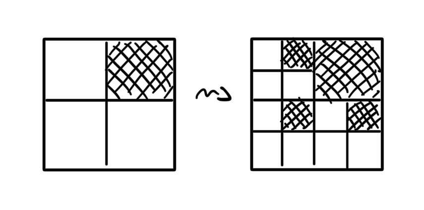
A screen is a term $$\lambda x.(x\ \textrm{tl}\ \textrm{tr}\ \textrm{bl}\ \textrm{br}),$$ where the terms tl, tr, bl, and br represent the top-left, top-right, bottom-left, and bottom-right quadrants of the image. Each of these terms can either be another screen, or a pixel.

A pixel is either on (white) or off (black). In its on state, a pixel is defined as the k combinator $$\textrm{w}=\lambda w\ b.w$$ In its off state, it’s the ki combinator $$\textrm{b}=\lambda w\ b.b$$ This decision was made for simplicity and could be any other state encoding, including ones of arbitrary size and color.

Example

Click the “Render” button to see the results.

• $\lambda \_\ x.(x\ \textrm{b}\ \textrm{b}\ \textrm{b}\ \textrm{b})$

• $\lambda \_\ x.(x\ \lambda y.(y\ \textrm{b}\ \textrm{w}\ \textrm{w}\ \textrm{b})\ \textrm{w}\ \textrm{w}\ \textrm{b})$

Rendering

For this project, I decided that the entire behavior of the screen is defined by a single closed lambda term. Upon execution of the renderer, this function gets applied to the default empty screen (four white squares). This enables the use of point-free/Tacit programming (e.g. using combinators), such that you don’t necessarily have to construct screens/colors at all.

Through slightly modified beta-reduction, the screen gets updated in-place while the term converges to its normal form. High rendering depths or diverging behavior may stop the renderer before convergence is reached.

Note that the renderer would also work with normal beta-reduction until convergence. The additional steps were only made to add support for in-place rendering of diverging terms.

Reduction

The in-place reduction-rendering works as follows (written as pseudo-Haskell using de Bruijn indices; actually implemented in JavaScript).

Figure out if a term looks like a screen:

isScreen (Abs (App (App (App (App (Idx 0) _) _) _) _)) = True
isScreen _                                             = False

Color the quadrants depending on pixel state (or grey if term is not yet figured out):

quadrantColor (Abs (Abs (Idx 1))) = White
quadrantColor (Abs (Abs (Idx 0))) = Black
quadrantColor _                   = Grey

Reduce to normal form (or loop endlessly):

nf (Abs t)   = Abs $ nf t
nf (App l r) = case nf l of
  Abs t -> nf $ subst t r
  t     -> App t (nf r)
nf t         = t

Reduce to weak-head normal form:

whnf (App l r) = case whnf l of
  Abs t -> whnf $ subst t r
  t     -> App t r
whnf t         = t

Reduce to screen normal form (either $\lambda x.((((x\ \textrm{tl})\ \textrm{tr})\ \textrm{bl})\ \textrm{br})$, $\lambda w\ b.w$, or $\lambda w\ b.b$):

snf t = case whnf t of
  Abs b -> case Abs $ whnf b of
    t@(Abs (Abs _)) -> nf t -- not a screen!
    t ->
      let go t | isScreen t = t
          go (App l r)      = case whnf l of
            (Abs t) -> go $ subst t r
            t       -> go $ App t (whnf r)
          go (Abs t) = go $ Abs $ whnf t
      in  go t
  _ -> error "not a screen/pixel"

Main reduction and rendering loop (assuming drawing functions that use and return some ctx):

reduce ((t, ctx) : ts) | quadrantColor t != Grey = reduce ts
reduce ((t, ctx) : ts) = if isScreen $ snf t
  then
    let (App (App (App (App _ tl) tr) bl) br) = t
    in  reduce ts
          ++ [ (tl, drawTopLeft ctx (quadrantColor tl))
             , (tr, drawTopRight ctx (quadrantColor tr))
             , (bl, drawBottomLeft ctx (quadrantColor bl))
             , (br, drawBottomRight ctx (quadrantColor br))
             ]
  else do -- this is pseudo-Haskell after all
    drawAt ctx (quadrantColor t)
    reduce ts

-- and, finally:
main t = reduce [(t, Ctx (canvas, width, height))]

See my reference implementation for more details.

Fractals

Sierpiński Triangle

We can’t trivially draw the classic “standing-up” Sierpiński triangle, since drawing the diagonals over square borders would get quite complex.

Instead, we can draw a rotated variant using a simple rewrite rule:

Translated to lambda calculus, we get the following:

$$\begin{aligned} \textrm{triangle}&=\lambda x.(x\ \textrm{triangle}\ \textrm{b}\ \textrm{triangle}\ \textrm{triangle})\\ \implies\textrm{triangle}'&=\lambda \_.(\textrm{y}\ \lambda t\ x.(x\ t\ \textrm{b}\ t\ t)) \end{aligned}$$

Or, golfed in binary lambda calculus to 51 bits:

000100011010000100000101010110110000010110110011010

Here, the rendering is stopped automatically after the smallest resolution of the canvas is reached. Note how the triangle structure appears even though we only ever explicitly draw black pixels. This is because the unresolved recursive $\textrm{triangle}$ calls get (temporarily) drawn as grey until they also get reduced. If the reduction wouldn’t be stopped, the canvas would slowly become black entirely.

T-Square

In each iteration, the T-Square adds new overlapping squares to the quadrants of every square already drawn. For lambda screen we can interpret this as a recursive split into smaller squares, where in each iteration one of the quadrants (depending on its position) gets drawn as black.

We can model this iteration as a mutual recurrence relation:

$$\begin{align*} \textrm{tl}&=\lambda x.(x\ \textrm{tl}\ \textrm{tr}\ \textrm{bl}\ \textrm{b})\\ \textrm{tr}&=\lambda x.(x\ \textrm{tl}\ \textrm{tr}\ \textrm{b}\ \textrm{br})\\ \textrm{bl}&=\lambda x.(x\ \textrm{tl}\ \textrm{b}\ \textrm{bl}\ \textrm{br})\\ \textrm{br}&=\lambda x.(x\ \textrm{b}\ \textrm{tr}\ \textrm{bl}\ \textrm{br})\\ \textrm{tsquare}&=\lambda x.(x\ \textrm{tl}\ \textrm{tr}\ \textrm{bl}\ \textrm{br}) \end{align*}$$

This relation can be solved using a variadic fixed-point combinator:

$$\begin{align*} \textrm{tl}'&=\lambda tl\ tr\ bl\ br.\lambda x.(x\ tl\ tr\ bl\ \textrm{b})\\ \textrm{tr}'&=\lambda tl\ tr\ bl\ br.\lambda x.(x\ tl\ tr\ \textrm{b}\ br)\\ \textrm{bl}'&=\lambda tl\ tr\ bl\ br.\lambda x.(x\ tl\ \textrm{b}\ bl\ br)\\ \textrm{br}'&=\lambda tl\ tr\ bl\ br.\lambda x.(x\ \textrm{b}\ tr\ bl\ br) \end{align*}\\ \textrm{mutual}=(\textrm{y*}\ \lambda a.(a\ \textrm{tl}'\ \lambda b.(b\ \textrm{tr}'\ \lambda c.(c\ \textrm{bl}'\ \lambda d.(d\ \textrm{br}'\ \textrm{nil})))))$$

Thus giving us the final term $\textrm{tsquare}'$, where the indices indicate the $n$th head selection of Church lists:

$$\textrm{tsquare}'=\lambda \_\ x.(x\ \textrm{mutual}_0\ \textrm{mutual}_1\ \textrm{mutual}_2\ \textrm{mutual}_3)$$

“Sierpiński Carpet”

The exact drawing of the Sierpiński Carpet is left as an exercise to the reader.

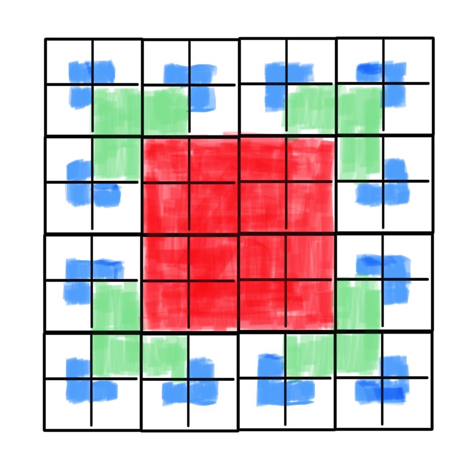
Since it’s a bit more straightforward, I decided to generate a slight variant¹ where each quadrant isn’t split into 9 but 4 quadrants per iteration.

Each new stable quadrant will be one of the following:

$$\begin{align*} \textrm{sub-tl}&=\lambda x.(x\ \textrm{b}\ \textrm{w}\ \textrm{w}\ \lambda y.(y\ \textrm{w}\ \textrm{w}\ \textrm{w}\ \textrm{b}))\\ \textrm{sub-tr}&=\lambda x.(x\ \textrm{w}\ \textrm{b}\ \lambda y.(y\ \textrm{w}\ \textrm{w}\ \textrm{b}\ \textrm{w})\ \textrm{w})\\ \textrm{sub-bl}&=\lambda x.(x\ \textrm{w}\ \lambda y.(y\ \textrm{w}\ \textrm{b}\ \textrm{w}\ \textrm{w})\ \textrm{b}\ \textrm{w})\\ \textrm{sub-br}&=\lambda x.(x\ \lambda y.(y\ \textrm{b}\ \textrm{w}\ \textrm{w}\ \textrm{w})\ \textrm{w}\ \textrm{w}\ \textrm{b}) \end{align*}$$

We again model the generation as a mutual recurrence relation:

$$\begin{align*} \textrm{tl}&=\lambda x.(x\ \textrm{tl}\ \textrm{tr}\ \textrm{bl}\ \textrm{sub-br})\\ \textrm{tr}&=\lambda x.(x\ \textrm{tl}\ \textrm{tr}\ \textrm{sub-bl}\ \textrm{br})\\ \textrm{bl}&=\lambda x.(x\ \textrm{tl}\ \textrm{sub-tr}\ \textrm{bl}\ \textrm{br})\\ \textrm{br}&=\lambda x.(x\ \textrm{sub-tl}\ \textrm{tr}\ \textrm{bl}\ \textrm{br})\\ \textrm{carpet}&=\lambda x.(x\ \textrm{tl}\ \textrm{tr}\ \textrm{bl}\ \textrm{br}) \end{align*}$$

Giving us, as before, the final term:

$$\begin{align*} \textrm{mutual}&=(\textrm{y*}\ \lambda a.(a\ \textrm{tl}'\ \lambda b.(b\ \textrm{tr}'\ \lambda c.(c\ \textrm{bl}'\ \lambda d.(d\ \textrm{br}'\ \textrm{nil})))))\\ \textrm{carpet}'&=\lambda \_\ x.(x\ \textrm{mutual}_0\ \textrm{mutual}_1\ \textrm{mutual}_2\ \textrm{mutual}_3) \end{align*}$$

There’s obviously huge potential for golfing the term size – so if you’re into that, have fun!

Cantor Dust

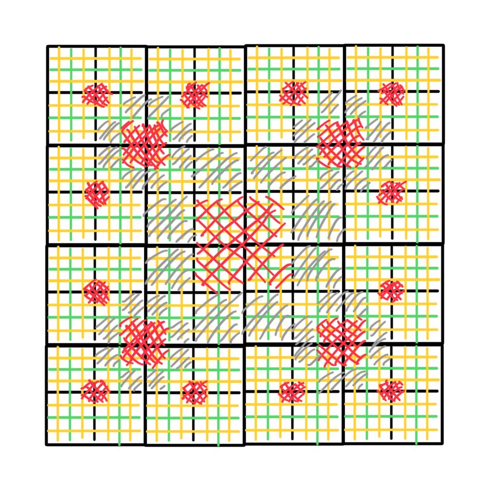
The Cantor dust is another great example of how infinitely detailed structures appear as unreduced (grey) quadrants when reduction inevitably gets halted.

In this case, a square gets recursively split into four new squares. Since we do the same split four times, we can construct the new quadrant using a $\textrm{quadruple}$ function:

$$\begin{align*} \textrm{quadruple}&=\lambda q\ x.(x\ q\ q\ q\ q)\\ \textrm{cantor}&=\lambda x.(\textrm{tl}\ \textrm{tr}\ \textrm{bl}\ \textrm{br})\\ \textrm{tl}&=(\textrm{quadruple}\ (\lambda x.x\ \textrm{cantor}\ \textrm{b}\ \textrm{b}\ \textrm{b})\\ \textrm{tr}&=(\textrm{quadruple}\ (\lambda x.x\ \textrm{b}\ \textrm{cantor}\ \textrm{b}\ \textrm{b})\\ \textrm{bl}&=(\textrm{quadruple}\ (\lambda x.x\ \textrm{b}\ \textrm{b}\ \textrm{cantor}\ \textrm{b})\\ \textrm{br}&=(\textrm{quadruple}\ (\lambda x.x\ \textrm{b}\ \textrm{b}\ \textrm{b}\ \textrm{cantor})\\ \end{align*}$$

After removing the recursive calls using $\textrm{y}$, we get

$$*\ *\ *$$

All of the examples above (and more) can also be found, rendered, and modified here.

Utilities

Lastly, here are some useful terms for experimentation (also available in the “template” preset).

Checking whether a pixel $p$ is black or white: $$\begin{align*} \textrm{w?}&=\lambda p.p\\ \textrm{b?}&=\lambda p.(p\ \textrm{b}\ \textrm{w}) \end{align*}$$

Inverting the state of pixel $p$: $$\textrm{invert}=\textrm{c}=\lambda p\ x\ y.(p\ y\ x)$$

Getting the term at a position $p$ of screen $s$:

$$\textrm{tl}=\lambda tl\ tr\ bl\ br.tl\quad \textrm{tr}=\lambda tl\ tr\ bl\ br.tr\\ \textrm{bl}=\lambda tl\ tr\ bl\ br.bl\quad \textrm{br}=\lambda tl\ tr\ bl\ br.br\\ \textrm{get}=\lambda p\ s.(s\ p)$$

Replacing a quadrant of screen $s$ with $q$:

$$\begin{align*} \textrm{tl!}&=\lambda s\ q.(s\ \lambda tl\ tr\ bl\ br\ x.(x\ q\ tr\ bl\ br))\\ \textrm{tr!}&=\lambda s\ q.(s\ \lambda tl\ tr\ bl\ br\ x.(x\ tl\ q\ bl\ br))\\ \textrm{bl!}&=\lambda s\ q.(s\ \lambda tl\ tr\ bl\ br\ x.(x\ tl\ tr\ q\ br))\\ \textrm{br!}&=\lambda s\ q.(s\ \lambda tl\ tr\ bl\ br\ x.(x\ tl\ tr\ bl\ q))\\ \end{align*}$$

Applying each quadrant of a screen $s$ to a function $f$:

$$\textrm{map}=\lambda f\ s.(s\ \lambda tl\ tr\ bl\ br.\lambda x.(x\ (f\ tl)\ (f\ tr)\ (f\ bl)\ (f\ br)))$$

Of course you could also use the definition of any function in bruijn’s standard library.

$$❦$$

Thanks for reading. Contact me via email. Support on Ko-fi. Subscribe on RSS. Discuss on Reddit and Hacker News. Follow on Mastodon.

I’ve also applied for a talk about this topic at GPN22 in Karlsruhe, so you may see me there as well.